A general election in the United Kingdom is less than nine months away. As the election nears we can expect more people to ask questions about the accuracy of opinion polling.
People – with pollsters not the least of them – display an endless capacity to worry about polling and whether it will “get it right”, and one new source of worry is multilevel regression and post-stratification (MRP), a way of producing small area estimates from large national samples.
MRP is becoming popular enough for it to get coverage in the national press, but the details of statistical models are always likely to be a niche concern.
One person who is concerned by MRP models is Peter Kellner. Peter has now written three separate blog posts, and in his most recent post threatens more. Here’s my attempt to head that off.
The argument
The strongest version of Peter’s argument against MRP is this:
- MRP estimates suggest a form of proportional swing, where Conservative losses are greater where they are defending larger vote shares;
- past British electoral history suggests that constituency-level swings between elections are uniform rather than proportional to the vote share a party was defending
- therefore MRP models are wrong
Both of the premises are broadly correct, but the conclusion does not follow. Let’s take the first claim, that MRP estimates reproduce a broadly proportional swing.
Here is a graph which uses the most recent seat-level estimates from Survation. On the horizontal axis, I’ve plotted the (notional) 2019 Conservative vote share. On the vertical axis, I’ve plotted the estimated change in vote share, if the election were held today.
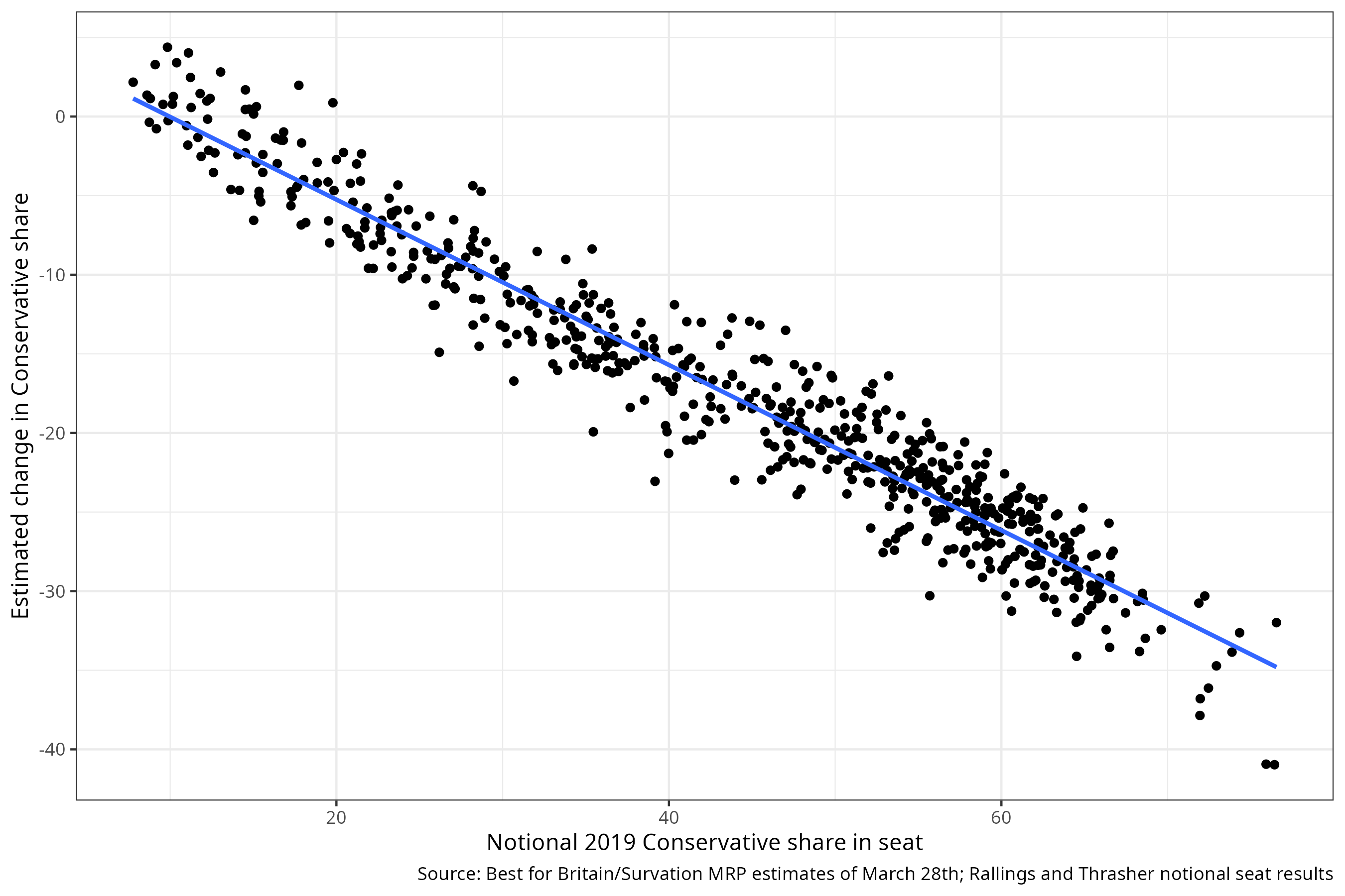
I’ve added a line of best fit, marked in blue. The fact that the blue line moves down as we move from left to right means that the fall in the Conservative vote will be greater the higher the Conservative vote share in 2019. If the swing were uniform, the line would not move down at all. These MRP estimates therefore more closely resemble proportional swing than uniform swing.
What about the second claim, that uniform national swing is a better model of between-election swings than proportional swing? There is, I’m afraid, no canonical reference to support this. It is instead generally accepted as an odd stylised fact about British electoral politics: “odd”, because it occasionally predicts negative vote share when a party’s share of the vote collapses, and “stylised”, because it neglects differences between the constituent nations of the UK.
I therefore think that both of Peter’s premises are correct. The problem is that the premises don’t imply the conclusion. MRP estimates are estimates of what would happen in an election if that election were held today. But an election is not being held today. People have not received campaign communications from the parties telling them that “Labour can’t win here”, or that it’s a two-horse race between red and blue. People are also far more likely to say that they don’t know how they will vote.
As we get closer to an election, and as people tune in to the campaign, their responses to surveys will change. These responses will start to incorporate new information, and we may see more voters making tactical choices as they learn more about party strength in their new or revised constituency. As survey responses change, so too do model predictions. The model will learn a new relationship between the constituency context and reports of voting intention.
It’s because “what people say to pollsters” changes the closer we get to the election that pollsters routinely claim that polling is a “snapshot, not a forecast”. Peter has been involved in polling for longer than I’ve been alive, and so he must be aware of this. But whatever affects ordinary polling also affects MRP estimates. In the case of ordinary polling, Peter would presumably be happy to say “the numbers from current polling look high, but these numbers come from a process which will deliver accurate numbers at the time of the election. We should therefore trust the process”. He should adopt the same approach for MRP.
A worked example
I have tried to make these arguments to Peter in the past when he has asked questions about the Survation model, but they have not convinced him. In this blog post I’ll therefore try a different tack, and show how a simplified version of an MRP model gives estimates that start proportional but become more uniform the closer we get to the election.
This model is so simple it can’t really be called an MRP model. An MRP model involves post-stratifying predictions – making predictions for different types, or strata, of respondents, and adding up predicted counts. One type might be 18 to 24 year men with A-levels who didn’t vote in the last election. The census and other administrative sources give us enough information to work out (roughly) how many people of that type there are in each constituency.
Although I tend to emphasise the role of post-stratification when explaining MRP to people, a lot of the work is actually done not by characteristics of people but by characteristics of areas. The most obvious area characteristic is simply “what proportion voted for each party last time”.
My “regression and prediction” model therefore includes only information on parties’ vote shares in the previous election, for constituencies in England. By limiting myself to England, I avoid having to deal with separate national swings in Scotland and Wales. By limiting myself to vote shares, I also avoid awkward questions about the different “vintages” of statistical information going in to my post-stratification frame.
To estimate this model, I’ll use vote intention reports from successive waves of the British Election Study. Because I’m not using any information about individuals, I’m going to add up the number of people in each wave and each constituency who say they’ll vote for a given party (or not vote at all). The outcome I’m trying to predict is therefore a vector of counts. Here’s what that looks like for Aldershot in the very first wave of the BES, way back in February 2014:
| DNV | Con | Lab | LDem | BP/Reform/UKIP | Green | DK | Other |
|---|---|---|---|---|---|---|---|
| 2 | 8 | 5 | 1 | 6 | 1 | 5 | 0 |
I’m now going to model the counts in Aldershot, and 533 other English constituencies, using four bits of information about each constituency:
- the Conservative share of the vote in the preceding election;
- the Labour share of the vote in the preceding election;
- the Liberal Democrat share of the vote in the preceding election;
- the Green share of the vote in the preceding election
The meaning of “the preceding election” changes depending on the wave. Waves 1 through 5 were collected before the 2015 election, and so the preceding election is the 2010 election.
Let’s focus on trying to predict outcomes in the first wave. Because I’m trying to model eight different things for each constituency, I have a number of different parameters that the model learns from the data:
- one intercept for each party, which gives me a baseline level of popularity when all of the other variables are zero
- Eight coefficients which tell me how much more likely each choice becomes when the Conservative share increases by one percentage point
- Eight coefficients which tell me how much more likely each choice becomes when the Labour share increases by one percentage point
- Eight coefficients which tell me how much more likely each choice becomes when the Lib Dem share increases by one percentage point
- Eight coefficients which tell me how much more likely each choice becomes when the Green share increases by one percentage point
In total, that’s 5 * 8 = 40 parameters to try and predict outcomes at this point in time. This is not a complicated model. By way of comparison, the Survation models will include just under ten thousand parameters.
Although the model is not a complicated one, 40 numbers is still a lot for people to take in, and these numbers are quantities known as log-odds ratios, which trip up even experienced statistical modellers. I’m therefore going to calculate, for this wave, the change in the Lib Dem share of the vote when the Liberal Democrat share last time round increases by one percentage point. I’m using the Liberal Democrats as an example because Lib Dem support is more concentrated, and more concentrated for idiosyncratic reasons, than almost any other party. The Liberal Democrats therefore suffer quite badly when models spread out their support across many seats.
If the model were to reproduce all the patterns of uniform national swing, then the change in the Lib Dem share of the vote associated with a one percentage point change should just be… one percentage point. Under uniform national swing, parties’ vote shares just move up and down according to some uniform shift which applies regardless of their vote share in each constituency. In the terms of the model, all the action is in the intercept, rather than the coefficients.
For the very first wave of the BES, before the 2015 election, the change in the predicted Lib Dem vote share, given a one unit increase in what happened last time, was one-third of a percentage point. This means that the Lib Dems will do less well than they otherwise might do in seats where they previously did well (because only one-third of their previous vote haul gets factored in). In other words, when this value is less than one, you get a more proportional swing.
Having calculated that quantity for the first BES wave, we can now step forward in time to the second BES wave, in May 2014, and re-run our model. The model is the same model as before, in the sense that it’s using the same variables as a basis for prediction, but it’s now working from new data. We can do what we did before, and calculate the change in the predicted Lib Dem share given a one unit change in what happened last time. And indeed, we can do that for every BES wave.
In the figure below, I’ve plotted all of these quantities, and their associated confidence intervals, in a graph. On the horizontal axis, we’ve got the approximate date of fieldwork of each BES wave. On the vertical axis, we’ve got the change in the Lib Dem vote share of a one unit increase in vote share in the previous election. Dashed vertical lines give the dates of the three elections in the period; the dashed horizontal line shows the one percentage point mark, or the point at which the model would (on average) start reproducing UNS for the Liberal Democrats.
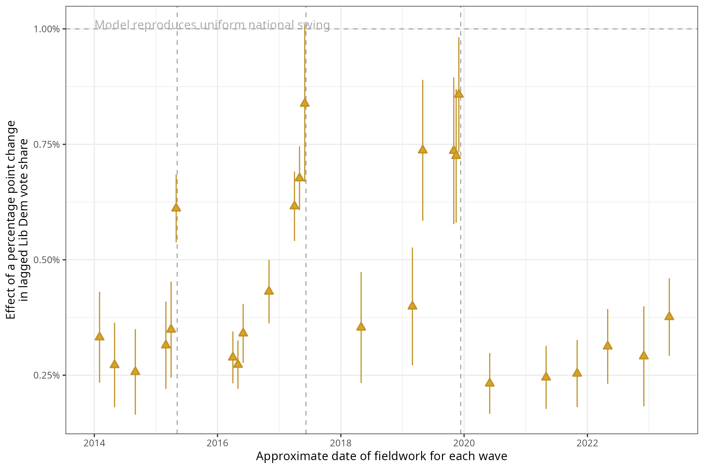
As you should be able to see, if we use the same model over these different waves, the results start out reproducing a very proportional swing, with each percentage point then translating to a third or half of a percentage point now. But around election times, the model suddenly learns that the association between then and now is much stronger.
In one wave – the campaign wave before the 2017 election – the confidence interval on this quantity just falls short of the magic UNS mark. This means that this simple model wouldn’t replicate UNS. But it is, of course, a simple model – and part of the reason we use MRP at all is because we don’t want to replicate UNS entirely, but allow for some subtler changes across different parties and across different local contexts.
In another wave – the wave before the 2015 election – the quantity is still quite low. But the 2015 election was the election where the considerable gains of the Rennard machine were wiped out following the Liberal Democrats’ experience of coalition and fairly ruthless targeting by the Conservatives of seats in the South West.
None of these quantities have changed because anything in the model changed: by construction, we’re using the same information to predict outcomes across each of these waves. Rather, it’s because the data the model was working with changed. The closer we get to an election, the more people’s self-reported vote intentions line up with the situation in their constituency.
If we knew that this election was going to be a repeat of the 2019 election, we could force these coefficients to be closer to the coefficient values we saw immediately before that election. This would turn an exercise into estimation into a blend of estimation and forecasting. But of course, we don’t know that this election will be a repeat of the last election. We don’t even know whether the value of this quantity will be anywhere in the range shown in the plot. In this election, we have to predict with notional figures of what would have happened if the 2019 election had been fought on 2024 boundaries. It seems unlikely that the relationship between past constituency strength and vote behaviour will be as strong when the constituencies have changed. There is, therefore, no easy way to “fix” this property of MRP estimates in order to bring them closer into line with expectations based on previous elections.
Conclusion
Thirty years ago, Andrew Gelman and Gary King wrote a paper with the title, “Why Are American Presidential Election Campaign Polls so Variable When Votes Are so Predictable?”. Their answer to the question they’d set themselves was this: although you could (at that time) predict the result of the election fairly well given the state of the economy (“fundamentals”), people weren’t paying attention to these things several months in advance of the election – or rather, they weren’t drawing connections between them. It wasn’t that the hundreds of millions spent on campaigns didn’t matter: it did matter, because it helped voters to connect the “fundamentals” to their vote choice.
We’re in a similar position with MRP. We have some MRP estimates of vote choice which contrast with what we know about inter-election swings. But we resolve this paradox by saying that campaigns matter to connect the fundamentals of constituency context to voter’s vote choices.
In this blog post I’ve demonstrated that the same MRP model will produce a swing that is closer to proportional several months away from an election, but rapidly approaches a more uniform swing the closer to an election the data is gathered. I’ve done this using publicly available data from the British Election Study; you can see the code I’ve used here. If you are criticising MRP models because they presently generate proportional swings, you need to be able to explain why we should expect uniform national swings right now, and why voters are able to internalize the tactical situation in their constituency several months before an election before parties have started actively campaigning.