The measurement of disproportionality in mixed member systems

Introduction

In the 2026 Scottish Parliament elections, the Scottish National Party won 44.6% of seats despite winning just 27.2% of the list vote. A gap of seventeen percentage points between vote and seat share might not seem exceptional by the standards of majoritarian elections, but the Scottish Parliament was elected by a form of mixed member proportional system which was designed to avoid the iniquities of first-past-the-post. If the disproportionality between seat shares and list vote shares is measured using the Gallagher index, then the 2026 election was the most disproportional Scottish Parliament election yet.

The reason the SNP won so many seats was that it performed much better in the nominal tier, winning 38% of the vote and 57 of 73 seats. It is common for large parties in mixed member systems to do better in the nominal tier than in the list tier, and we can give good reasons why: supporters of these parties often lend or rent out their vote to other parties (Meffert and Gschwend 2010; Gschwend et al. 2016). The list vote, despite being cast in a proportional tier, ends up being the less sincere and more strategic vote.

Despite the nominal tier vote being at least as sincere as the list, almost all¹ measures of disproportionality for mixed member systems are based on the share of the vote won in the list tier of the vote. For example: Linhart et al. (2019) compare levels of disproportionality using the Gallagher index and the list share of the vote. They do so even though they study several cases where the list vote was clearly strategic, including the notorious 2005 Albanian election, where the Democratic Party encouraged its supporters to vote for smaller satellite lists (Bochsler 2012), and where the party won 40% of seats on 7.7% of the list vote. The abuse of the system can surely have no defenders – but it does seem absurd that this measure of disproportionality does not depend at all on whether the Democratic Party won 7.7% of the votes in the nominal tier or the 44% it did in fact win.

In this note, I set out a way to measure disproportionality in mixed electoral systems which takes into account both nominal and list votes. This measure extends the Sainte-Laguë index, the disproportionality index which takes most seriously the element of unfairness present in seats-votes disproportionality. The measure is based on different voter types, defined by the party or parties each voter voted for across multiple tiers. Where all voters vote sincerely for the same party across both tiers, the measure collapses to the traditional Sainte-Laguë index. Where voters split their vote, the measure incorporates the electoral success of voted-for parties at both levels. The index shows that basing disproportionality just on the list share of the vote exaggerates the disproportionality found in mixed member systems.

Problems with calculating disproportionality on the basis of the list share

There are at least three reasons why calculating disproportionality on the basis of the list vote alone – or what I’ll call standard practice – is bad. These reasons apply to all commonly used indices of disproportionality.

First, standard practice does not take account of the fact that the list share of the vote may not be principal determinant of seat shares. In particular, standard practice makes little sense in parallel systems where a majority of seats are awarded based on the nominal tier, or in compensatory systems where the nominal tier makes up more than three-quarters of the total seats (Bochsler 2023, 102557). Japan is an example of a parallel system where the nominal tier is more important (289 of 465 seats awarded in the nominal tier); Korea is an example of a notionally compensatory system where the proportional tier makes up just 15% of the legislature. These systems are not designed to make seat shares fully match list shares, and so presenting information on the gap between list shares and seat shares seems to miss the point. For these systems we might consider calculating disproportionality on the basis of the nominal tier share of the vote, but this would create a demarcation problem (when is the nominal tier share so large that the relevant vote share is the nominal tier share rather than the list tier share?)

Second, standard practice does not take account of the fact that the set of parties competing in the nominal and list tiers may vary for reasons good or bad. Take as an example the Non-Partisan Solidarity Union in Taiwan, which in the 2012 election ran only in single member districts, winning two seats. Because its list vote share was technically zero, the gap between its seat and vote share contributes significantly to overall disproportionality as measured by the Gallagher or Loosemore-Hanby indices. Worse still, the fact that the party won seats on zero percent of the vote creates a division-by-zero error in the formula used to calculate the Sainte-Laguë index, meaning that disproportionality is undefined!

Nominal and list-tier parties may differ for bad reasons. Decoy lists – where a party runs constituency candidates in a separate list to frustrate compensatory mechanisms in the list tier – are commonly held to be a bad thing (Bochsler 2012). These lists are bad because they frustrate the intent of the electoral law, but they are also bad because they make it harder to calculate a meaningful measure of disproportionality if the decoy list technically has negligible list vote share.

Third, standard practice ignores the fact that some voters “lend” or “rent out” their vote precisely because there is another approved party which is likely already to benefit from the electoral system (Meffert and Gschwend 2010, 2011; Gschwend et al. 2016). CDU/CSU voters in Germany often lend their vote to the FDP so that it can pass the electoral threshold (Roberts 1988); SNP voters in Scotland similarly lend their vote to the Green party so that they can broaden the set of pro-independence parties. Should that strategy fail – as it did in the 2013 German elections – then it would seem strange to regard those lent votes as major contributors to disproportionality: the people who cast those lent votes already got a good return on their nominal tier vote.

Sadly it is not possible to remedy these problems easily. We can’t calculate separate indices of disproportionality for the different tiers and aggregate these together: the disproportionality in a nominal tier will advantage one set of parties, whilst the disproportionality in a compensatory tier will advantage a different set of parties, and because disproportionality is not signed, these two disproportionalities will add to something greater than any plausible measure of overall disproportionality.

We also can’t average the vector of vote shares across the two tiers. Averaging shares across the two tiers makes sense, but it fails to deal with the problem of parties that don’t run in both tiers, and parties that create decoy lists. It also fails to address “rental” mechanisms which mean that the vote share in one tier may be “low” precisely because support is strategically being directed to the other tier.

An extension to the Sainte-Laguë index

I suggest extending an existing measure of disproportionality (the Sainte-Laguë index) to deal with the problem of multiple tiers. Because the Sainte-Laguë index can be represented as though it aggregated over voters rather than parties, it can be extended to analyse disproportionalities across multiple voter types, where a voter type is defined by the set of parties voted for across multiple tiers. This party/party-supporter duality allows me to combine the two tiers and present a measure of disproportionality that summarizes inequality amongst voters and disproportionality between parties.

The Sainte-Laguë index has two inputs: a vector of vote shares \(v\), and a vector of seat shares \(s\). The index can be written using two formula which look different but give identical results. The index can be written using squared differences between seat and vote shares:

\[ D_{SL} = \sum_i^N \frac{(s_i - v_i)^2)}{v_i} \tag{1}\]

where each party is indexed by \(i\), and the summation runs over all parties \(i = 1, ... N\). This way of writing the index makes the index resemble the chi-squared index used to measure association.

Alternately, the index can be written as a weighted average of advantage ratios. The advantage ratio for a party, \(A_i\), is equal to its seat share divided by its vote share: \(A_i = \frac{s_i}{v_i}\). Because shares always sum to one, the weighted mean advantage ratio across all parties must equal one. Departures from an advantage ratio of one therefore indicate disproportionality. The index is:

\[ D_{SL} = \sum_i^n v_i (A_i - 1)^2 \tag{2}\]

Writing the Sainte-Laguë index in the form given by Equation 2 allows us to think about what an extended index might look like if voters, not parties, were the unit of account (Van Puyenbroeck 2008). Rather than speak of individual voters, I am going to aggregate and deal with voter types.

A voter type is defined by the set of parties they vote for across multiple tiers. The voter who votes for the CDU in the constituency vote and for the FDP in the list vote is one type. So too is the voter who votes for the SPD in the constituency vote and the AfD in the list vote. The voter who votes for the CDU in both the constituency vote and in the region vote is a particular type of voter: a straight-ticket voter.

Voter types are defined by unordered sets of parties, and don’t take account of which vote was cast for which party. This means that the voter who votes for the CDU in the constituency vote and the FDP in the list vote is of the same type as the voter who votes for the FDP in the constituency vote and the CDU in the list vote.

If there are \(n\) parties competing, then the number of voter types is equal to the square of the number of parties. This is the number of logically possible voter types, but not all of these types are politically plausible: there are some voters who voted for the SPD in the constituency vote but AfD in the list vote, but this type is rare.

Having introduced the language of voter types, I’ll now make a further conceptual shift, and talk about advantage ratios for voter types rather than parties. I’m going to stipulate that the advantage ratio for a voter of type \(t\) is equal to the average of advantage ratios of the parties that they supported, and that the advantage ratio for each party is now calculated based on the seats they won, divided by the proportion of voters who voted for them on either vote.

Formally,

\[ A_t = \sum_{i \in t} \frac{1}{2} \frac{s_i}{q_i} \tag{3}\]

where \(i\) is a party that makes up voter type \(t\), and where \(q_i\) is the proportion of people that voted for party \(i\) in either ballot. The proportion \(q_i\) is always greater than a party’s list share or their nominal tier share, and the sum of all values of \(q_i\) ranges between 100% (all voters are sincere and do not split their votes) to 200% (all voters split their ballot).

It should be clear from these definitions that we cannot work out how many people belong to each different voter type from the results data alone. If a party wins 10% of the constituency vote and 20% of the regional vote, then it’s likely that the overwhelming share of the constituency voters also gave their regional vote to that party, but even that is not guaranteed, and we have no way of knowing where the other ten percentage points came from.

I therefore work with survey data to develop this extended measure of disproportionality. My example is drawn from the 2021 Scottish Election Study. The figures in this section are based on the post-election survey wave, except that the survey weights for respondents have been raked so that the sample proportions of nominal and list votes for each party exactly match the reported results.

Table 1: Information on voter types. Cell entries give the proportion who gave votes to both the column and the row party. Some cells highlighted for illustration.

Party	Con	Green	Lab	LDem	Other	SNP
Con	18.06%	0.05%	5.33%	1.78%	1.62%	0.47%
Green	.	0.62%	0.90%	0.43%	0.09%	6.70%
Lab	.	.	14.45%	1.67%	0.85%	1.86%
LDem	.	.	.	3.57%	0.26%	0.71%
Other	.	.	.	.	0.44%	1.96%
SNP	.	.	.	.	.	38.16%

Table 1 gives information on the break-down of types in the 2021 election. The largest single type of voter (38.16% of all voters) is the voter who cast their vote for the SNP in both contests. There are large entries on the diagonals, which represent straight-ticket voters, but some of the off-diagonal entries are clearly relevant, like the 7% of voters who split their votes between the SNP and the Greens.

We can use this information to calculate advantage ratios for different voter types:

• for the voter type {SNP}: the number of seats won by the SNP in the 2021 election was \(64 / 129 = 0.496\); the proportion of people who voted for the SNP on either ballot was 0.499 (this being the sum of all entries in the yellow column); the party’s advantage ratio is therefore 0.994.

• for the voter type {SNP, Green}: the advantage ratio for the SNP is as previously calculated. The advantage ratio for the Green party is their seat share (6.2%) divided by the proportion who voted for them on either ballot, or 0.0879153 (this being the sum of all entries in the L-shaped group of cells with a green border); the party’s advantage ratio is therefore 0.705; the average of these two advantage ratios is 0.85

Because \(q\) sum to more than 100%, the average advantage ratio is less than one. That means we can’t apply the Sainte-Laguë formula above in Equation 2, which relies on the accounting identity that the population weighted advantage ratio is one. We must normalize by dividing by the share-weighted average of advantage ratios, or 0.827. Call this adjusted figure \(\tilde{A}\). We can then use \(\tilde{A}\) in Equation 2, and replace the vote share with the proportion of voters in each type.

Formally,

\[ D_{SL}^{\ast} = \sum_t^T p_t (\tilde{A_t} - 1)^2 \tag{4}\]

where \(\tilde{A_t} = \frac{A_t}{\bar{A}}\), \(\bar{A} = \sum_t^T p_t A_t\), and \(A_t\) is as described in Equation 3.

Given Equation 4, then disproportionality in the 2021 Scottish Parliament election was
5.3%, rather than the value of 0.069 that one would get by following standard practice and calculating the Sainte-Laguë index using the list share alone. Extending the Sainte-Laguë index in this allows us to recognize that many people voted for the SNP in the nominal tier and lent their votes to other parties in the list tier, and that therefore the SNP is not as over-represented as one might think – except that now we must say, “voter types involving the SNP” are not as advantaged as the list share alone would suggest.

Comparative evidence

We can repeat this exercise for other countries which use mixed systems. Here I draw on the Comparative Study of Electoral Systems Integrated file and two elections from module 6 of the CSES. I am able to use all mixed elections save one: the 2005 survey of Albanian voters does not include anyone who voted for some seat-winning parties. As such, I am unable to construct the joint distribution for all relevant parties for this election. I return to this issue in the conclusion.

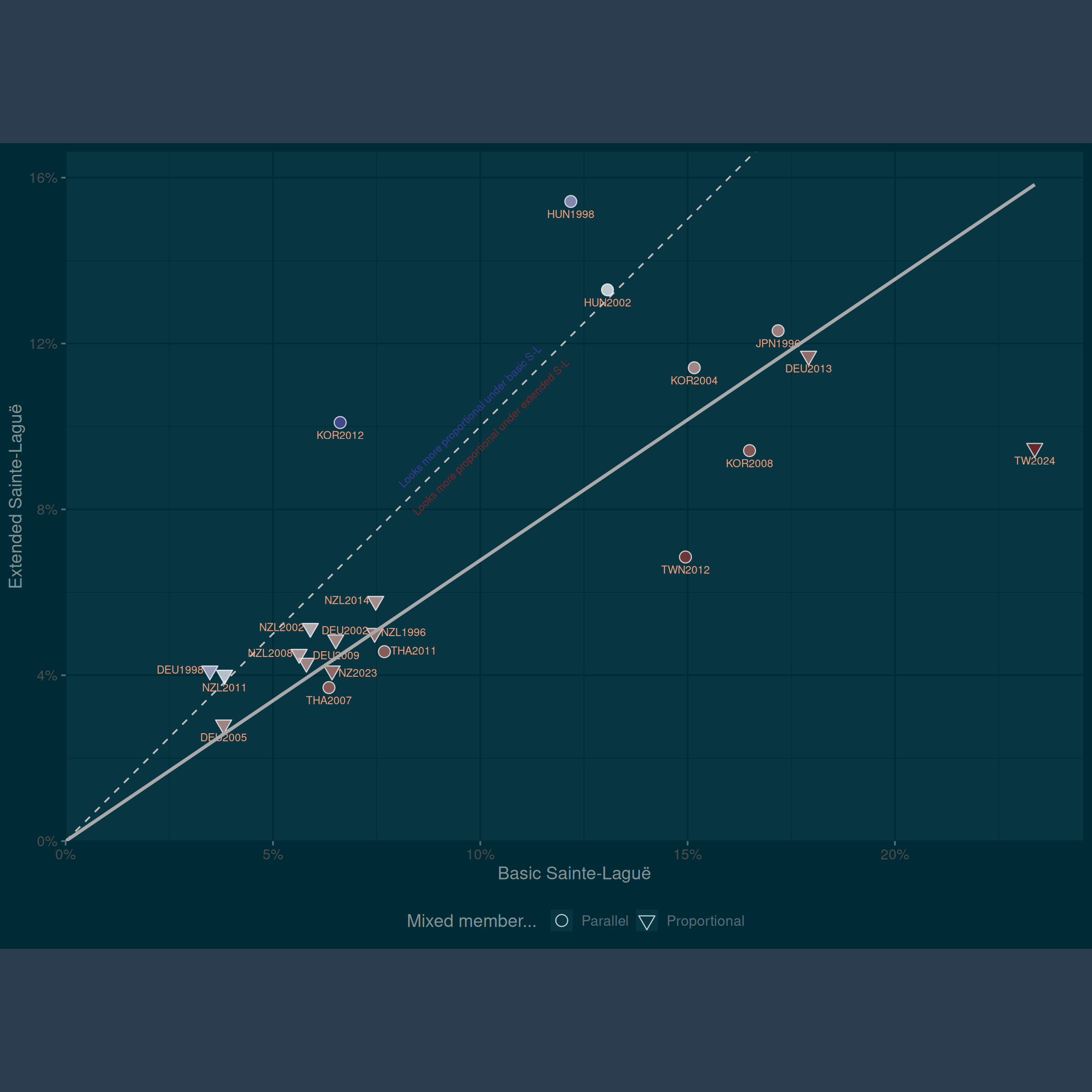
Figure 1 shows the values for all the mixed member elections in the CSES. In general, disproportionality under the extended Sainte-Laguë index is around two-thirds of disproportionality under the basic Sainte-Laguë index. Most elections have lower values under the extended index, but there are some exceptions. I discuss the Korean case below in more detail, as it is the most obvious exception to the pattern. Other elections where the extended Sainte-Laguë index exceeds the basic index result from complexities of the nominal tier: in Hungarian elections, the higher figure under the extended Sainte-Laguë arises because of disproportionalities in the two-round nominal tier, where first-round shares can be a poor guide to seat outcomes.

The two measures are visibly correlated (\(r = 0.725\)), and so elections which have high disproportionality based on the list votes alone are also likely to have high disproportionality based on this extended index – but the overall levels are lower. This in turn has implications for the level of disproportionality achieved in mixed systems compared to other simpler systems.

Whether the mixed system is mixed member proportional or mixed member parallel does not seem to affect the relationship between basic Sainte-Laguë and the extended version. Mixed member parallel systems generally have higher disproportionality, and so they are further to the right side of the graph. However, mixed member proportional systems can also have high disproportionality, as in Germany in 2013, when the FDP, AfD, and Piraten all fell foul of the five percent threshold. That disproportionality concerned the proportional tier alone, and this election result looks disproportional on either the basic Sainte-Laguë index or the extended version.

Figure 1: Scatter-plot showing values of the ordinary Sainte-Laguë index calculating using vote shares from the proportional tier, and the extended Sainte-Laguë using information from votes in both tiers. Countries below the 45 degree line have lower values under the extended index.

We can also compare the extended version of the Sainte-Laguë index that I have argued for to the simpler version which involves averaging over vote shares in the nominal and list tiers before calculating disproportionality. This is shown in Figure 2. These two measures are more strongly correlated (\(r = 0.878\)), but there are differences in the levels. Levels of disproportionality under the extended Sainte-Laguë index are generally lower, and are on average around 87.3 percent of the values of the index when averaging over nominal and list tier votes.

Figure 2: Scatter-plot showing values of an ’averaged’Sainte-Laguë index calculating using the average of vote shares from the nominal and list tiers, and the extended Sainte-Laguë using information from votes in both tiers. Countries below the 45 degree line have lower values under the extended index.

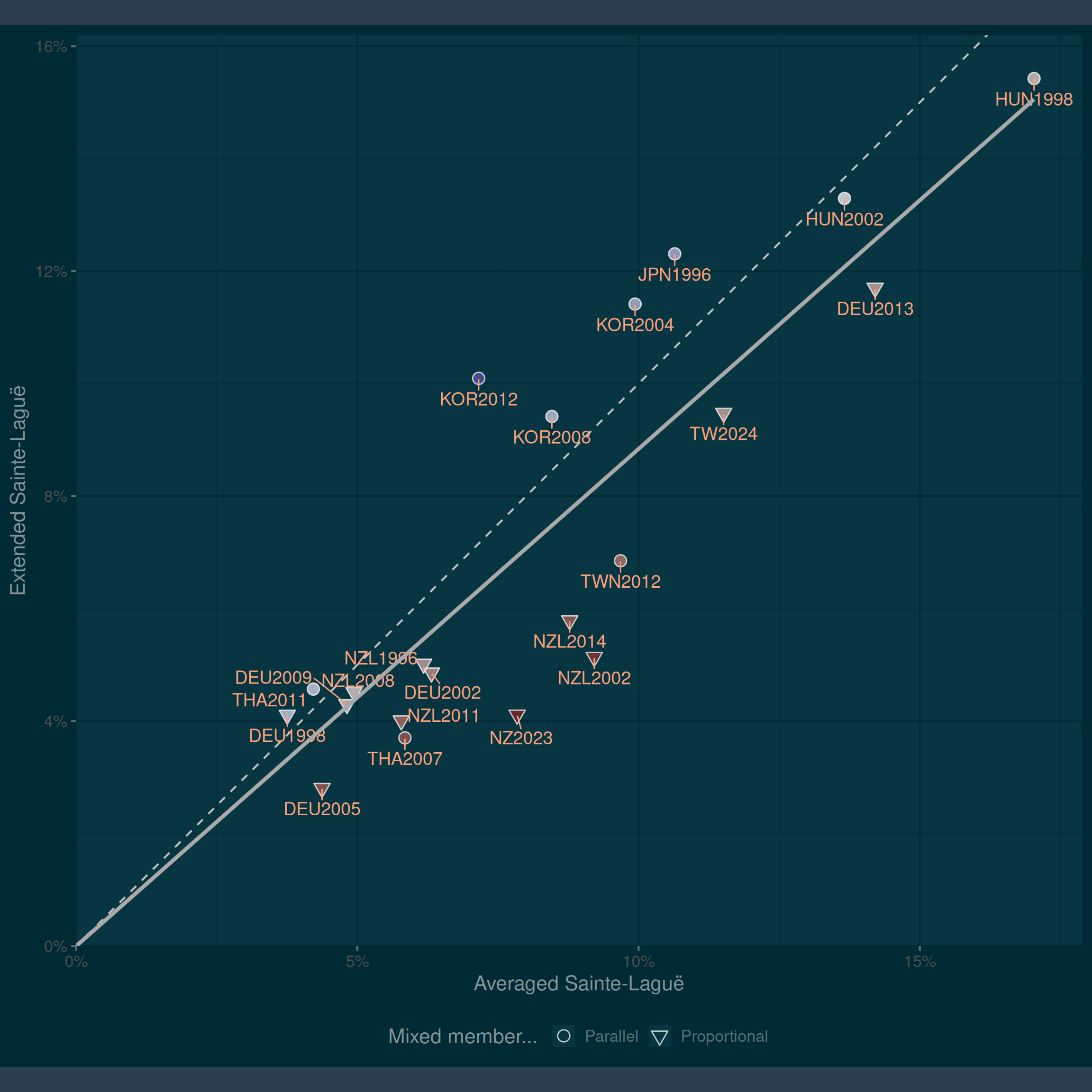
Whether we compare the extended Sainte-Laguë to the basic Sainte-Laguë index or to a version which averages over list and nominal shares, there are pairs of countries which have very different values on the two indices. The most obvious contrast is between New Zealand in 2023 and South Korea in 2012. These two elections were equally disproportional if we are to judge by the standard Sainte-Laguë index: the values are almost identical (0.066 for Korea, 064 for New Zealand). However, the extended index suggests that the South Korean result was much more disproportional. Why is this?

The answer lies in a combination of the gap between list and nominal shares, the dispersion of advantage ratios; and the size of split-ticketing groups which choose “poorly”. First, note that in the 2012 Korean election, the gap between the list tier share and the nominal tier share was small for the two largest parties – of the order of a percentage point. The extended Sainte-Lagüe index can make an outcome that seems disproportional on the basis of the list tier look better by incorporating information from the nominal tier. Here, there is no gap to make good. Second, note that the Korean system is heavily majoritarian – the nominal tier contributes 85% of seats. This means that the votes-seats curve is extremely steep at its inflection point. The contrast is with the New Zealand system which has a discontinuity in the votes-seats curve at the threshold of five percent, but is otherwise fairly smooth. Whether they lend their votes to the Greens, the ACT, or NZ First, voters are similarly treated, even though these parties differ in vote share by five to six percentage points. Third, although many voters in the Korean election were straight-ticket voters, a sizeable proportion of Saenuri and Democratic United Party voters experimented with other parties. Because the votes-seats curve is so steep, any defection from one of the two big parties means that these voters advantage ratio couples one fairly good advantage ratio to one fairly disastrous advantage ratio. In other words, the extended Sainte-Laguë index shows that in a more majoritarian mixed system, trying to split your vote risks wasting at least one vote. The difference in values is therefore indicative of the difference in the two systems which, although both formally of the same mixed member proportional type, differ substantially in their composition.

Conclusions

In this note I’ve introduced an extension of the Sainte-Laguë index which allows the measurement of disproportionality across multiple votes given information on the joint distribution of those votes.

This index has several desirable features. First, it allows us to incorporate information from both votes cast by voters, rather than privileging one vote and ignoring the other. Second, the index collapses to the normal Sainte-Laguë index if all voters are straight-ticket voters. Third, the index deals with decoy lists by exploiting the empirical overlap between nominal slates and upper-tier lists.

The major disadvantage of the index is that it requires information on the joint distribution of votes across tiers. In this note I have used survey information to construct that joint distribution, but I have also noted that in one case (Albania 2005) the survey data was not detailed enough to construct the marginal distributions for at least one seat-winning party. I would suggest that estimating the joint distribution of votes is a basic descriptive task for anyone involved in studying elections in countries which use mixed systems, and so this information ought to be available. If it is not available then it would in principle be possible to estimate the joint distribution using ecological inference, particularly where electoral results are available at a very granular level.

This extension to the Sainte-Laguë index is not the only possible way of extending the index. In particular, I have made some design choices that seemed to me appropriate, but that are not the only valid choices. I have defined voter types as the unordered set of parties supported by each voter, rather than the set ordered by tier. In some senses, the voter who votes for the CDU/CSU in the nominal tier and lends their vote gets the same representation as the voter who votes the other way around, but it seems odd to say that they are equally advantaged. Paying attention to ordering raises the question of whether we should attach the same weight to advantage ratios for “list-tier” parties and “nominal tier” parties. Our present standard for calculating disproportionality attaches zero weight to the constituency tier, and I think that is wrong, but it does not follow from this that the best weighting is an equal weighting. I have not gone beyond equal weighting because unequal weighting seems to move us beyond disproportionality and into an assessment of how well election outcomes match voters’ cardinal utility over parties, and that is definitely a much bigger topic than can be handled here (Monroe 1995; Blais et al. 2022).

References

Blais, André, Eric Guntermann, Vincent Arel-Bundock, Ruth Dassonneville, Jean-François Laslier, and Gabrielle Péloquin-Skulski. 2022. “Party Preference Representation.” Party Politics 28 (1): 48–60.

Bochsler, Daniel. 2012. “A Quasi-Proportional Electoral System ‘Only for Honest Men’? The Hidden Potential for Manipulating Mixed Compensatory Electoral Systems.” International Political Science Review 33 (4): 401–20.

Bochsler, Daniel. 2023. “Balancing District and Party Seats: The Arithmetic of Mixed-Member Proportional Electoral Systems.” Electoral Studies 81: 102557.

Gschwend, Thomas, Lukas Stoetzer, and Steffen Zittlau. 2016. “What Drives Rental Votes? How Coalitions Signals Facilitate Strategic Coalition Voting.” Electoral Studies 44: 293–306.

Linhart, Eric, Johannes Raabe, and Patrick Statsch. 2019. “Mixed-Member Proportional Electoral Systems–the Best of Both Worlds?” Journal of Elections, Public Opinion and Parties 29 (1): 21–40.

Meffert, Michael F, and Thomas Gschwend. 2010. “Strategic Coalition Voting: Evidence from Austria.” Electoral Studies 29 (3): 339–49.

Meffert, Michael F, and Thomas Gschwend. 2011. “Polls, Coalition Signals and Strategic Voting: An Experimental Investigation of Perceptions and Effects.” European Journal of Political Research 50 (5): 636–67.

Monroe, Burt L. 1995. “Fully Proportional Representation.” American Political Science Review 89 (4): 925–40.

Roberts, Geoffrey K. 1988. “The ‘Second-Vote’campaign Strategy of the West German Free Democratic Party.” European Journal of Political Research 16 (3): 317–37.

Tanács-Mandák, Fanni, and Attila Horváth. 2025. “The ‘Hacking’ of a Mixed Electoral System: A Case Study of Hungary.” Public Choice 204 (1): 75–99.

Van Puyenbroeck, Tom. 2008. “Proportional Representation, Gini Coefficients, and the Principle of Transfers.” Journal of Theoretical Politics 20 (4): 498–526.

Footnotes

1. There are some papers which calculate disproportionality in different ways, but this is usually only intended as a way of decomposing electoral advantage, rather than stipulating a measure of disproportionality as such. Tanács-Mandák and Horváth (2025), for example, measure “total disproportionality” in Hungary by comparing seat share to list share, but also compare the share of list votes to the share of list seats, and the share of list votes to the share of SMD seats, a measure which makes little sense in the context of the measurement of disproportionality but which helps explain a great deal about Fidesz’ advantage under the Hungarian system.