tl:dr version If you predict a leftward shift when you previously saw a rightward shift, you’re just predicting regression to the mean, not conscious zig-zagging.
Ian Budge’s 1994 article “A new spatial theory of party competition” belongs to that efflorescence of research into party systems in the 1990s, when the number of electoral democracies was growing, not shrinking, and when the CD-ROM was the shiny new solution to data interchange.
The article is today best known for introducing different policy rules followed by parties, prefiguring much more recent research on agent-based models for party competition.
There is, for example, the “stay-put” model (Laver and Sergenti’s “Sticker” rule), where the party always adopts the same position, and a “past results” model, which is similar to the “Hunter” rule).
There is also an “alternation model”, which says that
“Parties alter priorities in different directions between each election. Operationally we expect this to give rise to a zig-zag pattern as leftward shift succeeds rightward shift and vice versa”
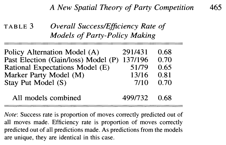
Not all of these rules apply to all parties, so Budge works out how many shifts each model successfully predicts. For the “alternation model”, he works out that the model predicts 68% of inter-election changes in party position.
This seemed very impressive to me when I first read it. If party shifts are either “right-ward” or “left-ward”, and if there are no good reasons to think that parties generally shift left-ward or right-ward, then a model where we guess the direction of the shift at random would give us a “percentage correctly predicted” of 50%. 68% is a lot more than 50%, so this seems like evidence that parties consciously zig-zag.
Unfortunately, the success of the model in predicting shifts doesn’t support a model of conscious zig-zagging – or rather, the model’s success is compatible with a much simpler model.
I’ll show this by simulation in R before I give the intuition (largely because I convinced myself in the same order).
A short simulation
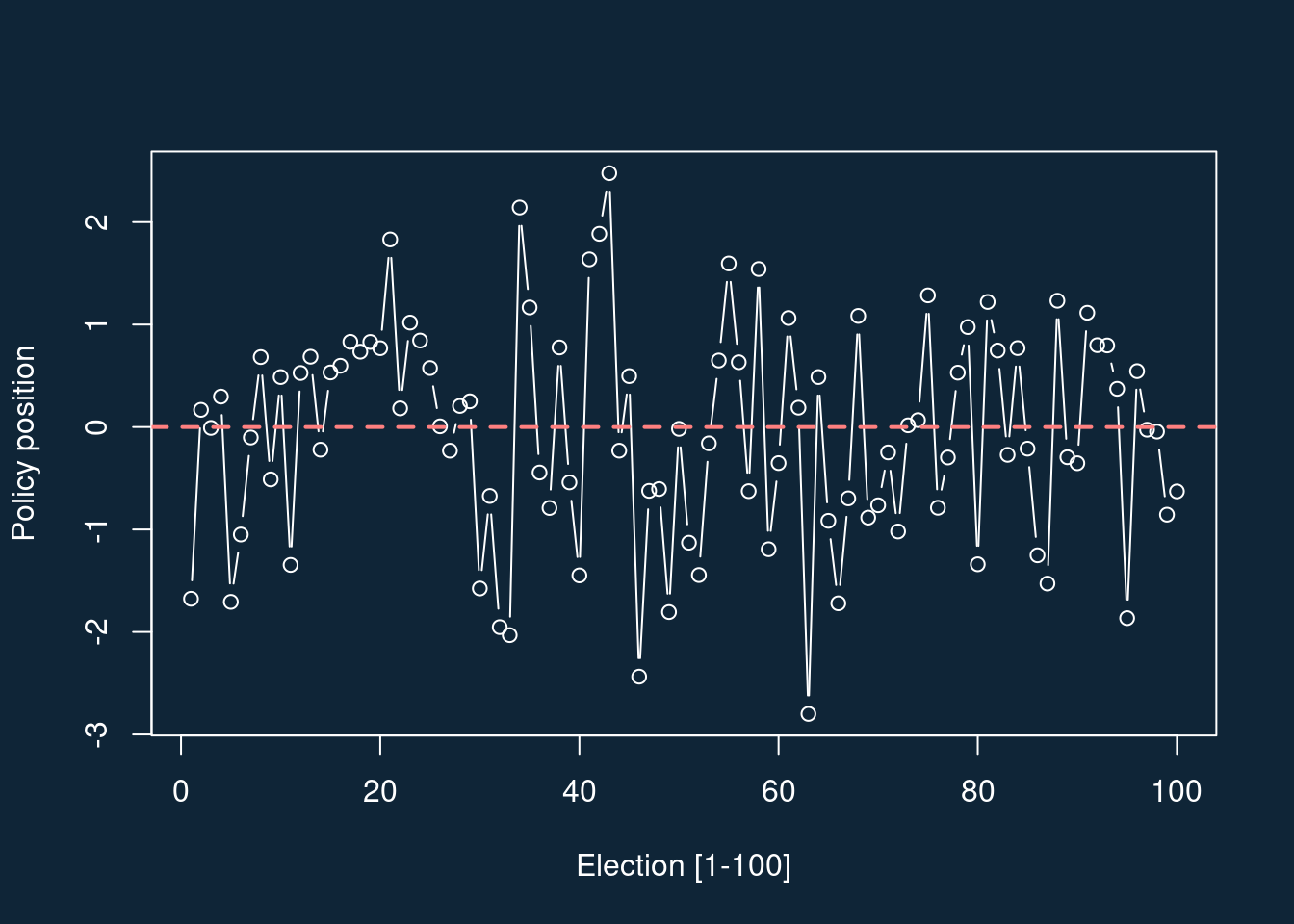
Imagine that parties always have the same position, but that this position is always measured with some noise. For convenience, let’s fix the party’s true position to zero.
tru <- 0Now let’s imagine there’s some error – a slip in communication, a missed phrase or two in a manifesto – which gives rise to a measured position. These errors are independent across multiple elections.1
set.seed(118)
nElex <- 100
err <- rnorm(nElex, mean = 0, sd = 1)
measure <- tru + err
We can store this in a data frame to keep things tidy.
dat <- data.frame(election = seq_len(nElex),
                  measure = measure)
Let’s work out the shift at each time. We’ll do this by creating a lagged version of the measure, and calculating the difference.
library(tidyverse)

dat <- dat |>
    mutate(last_time = lag(measure),
           delta = measure - last_time,
           shift = ifelse(delta > 0, "right", "left"))

head(dat)
election measure last_time delta shift
1 1 -1.676079782 NA NA <NA>
2 2 0.167651720 -1.676079782 1.8437315 right
3 3 -0.008545182 0.167651720 -0.1761969 left
4 4 0.296888139 -0.008545182 0.3054333 right
5 5 -1.706489201 0.296888139 -2.0033773 left
6 6 -1.049094451 -1.706489201 0.6573947 rightHere’s what those policy positions look like over time:
Now we need to make our prediction. We’re going to base this on the previous shift, so we’ll need to create a lagged version of this variable too.
dat <- dat |>
    mutate(last_shift = lag(shift))
Now we create our prediction.
dat <- dat |>
    mutate(pred = ifelse(last_shift == "left",
                         "right",
                         "left"))
How well do we do?
dat <- dat |>
    mutate(correct = (pred == shift))

mean(dat$correct, na.rm = TRUE)
[1] 0.6122449Huh – we’ve ended up with something close to the figure Budge got, and much higher than 50%. Is that just a fluke? Can we do this again?
In the code below, I create a short function which repeats the exercise for a given number of elections. I set that number of 431, because that’s the number of shifts Budge looks at. I then repeat this simulation of 431 elections 1,000 times.
### Let's wrap this up as a function
sf <- function(nElex) {
    measure <- 0 + rnorm(nElex)
    dat <- data.frame(election = seq_len(nElex),
                      measure = measure) |>
        mutate(measure.l1 = lag(measure),
               delta = measure - measure.l1,
               shift = ifelse(delta > 0, "right", "left"),
               shift.l1 = lag(shift)) |>
        mutate(pred = ifelse(shift.l1 == "left",
                             "right",
                             "left"))
    return(mean(dat$pred == dat$shift, na.rm = TRUE))
}

res <- replicate(1000, sf(431))
We can plot the distribution of success rates, and overlay the rate Budge found (291/431 = 67.5%).
par(bg = "#0f2537", fg = "white", col.lab = "white", col.axis = "white",
    col.main = "white", col.sub = "white")
hist(res,
     main = "Distribution of success in predicting shifts",
     sub = "Red line shows rate from Budge (1994)",
     xlab = "Success rate (%)")
abline(v = 291/431, col = "#ff8080", lwd = 2)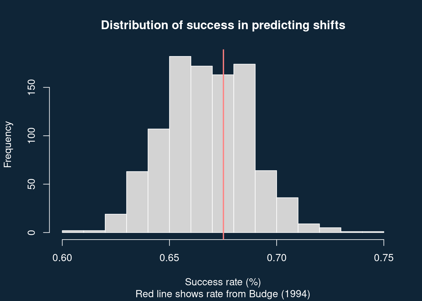
Why, when the true process is one of “no change, only error”, do we do so well in “predicting” party shifts between elections?
It’s that well-known-but-rarely-understood phenomenon of “regression to the mean”. (The Wikipedia article is really well written, so if you haven’t read it already, do so now). Regression to the mean is usually discussed in the context of continuous values: if I score high on one test (to use the same example as the Wikipedia entry), I’ll probably score less well on the next test. Here we don’t have continuous values, only categories, but those categories play a similar role.
Suppose we see a right-ward shift between two elections. That probably means that the measurement error this time was positive. (think: if the measurement error was negative, then we could only get a right-ward shift if the previous measurement error was even more negative). If we predict a left-ward shift, we’re predicting that the next measurement error will be less extreme – in this case, less positive. This is just another way of saying that our “zig-zag” prediction is just predicting a regression to the mean.
I don’t know why this didn’t occur to Budge. I only realized this because I tried to simulate the underlying process. It’s possible that Budge was thinking of a different kind of randomness – a random walk, where party positions are not fixed, and where the probability of successfully predicting the next shift under a null model really is fifty percent (see code below). This kind of random walk has been discussed in the literature, but given the short time series involved (particularly at the time Budge was writing), it can be hard to distinguish between the two.
The lesson of this? Always ask whether the number you’ve been quoted is a big or small number, and whether you could reach that same number by simulating a much more boring process than the one you’re asked to believe in.
Bonus random walk code
sf <- function(nElex) {
    require(tidyverse)
    measure <- cumsum(rnorm(nElex))
    dat <- data.frame(election = seq_len(nElex),
                      measure = measure) |>
        mutate(measure.l1 = lag(measure),
               delta = measure - measure.l1,
               shift = ifelse(delta > 0, "right", "left"),
               shift.l1 = lag(shift)) |>
        mutate(pred = ifelse(shift.l1 == "left",
                             "right",
                             "left"))
    return(mean(dat$pred == dat$shift, na.rm = TRUE))
}


res <- replicate(1000, sf(431))
par(bg = "#0f2537", fg = "white", col.lab = "white", col.axis = "white",
    col.main = "white", col.sub = "white")

hist(res,
     main = "Distribution of success in predicting shifts",
     sub = "Results from a random walk model",
     xlab = "Success rate (%)")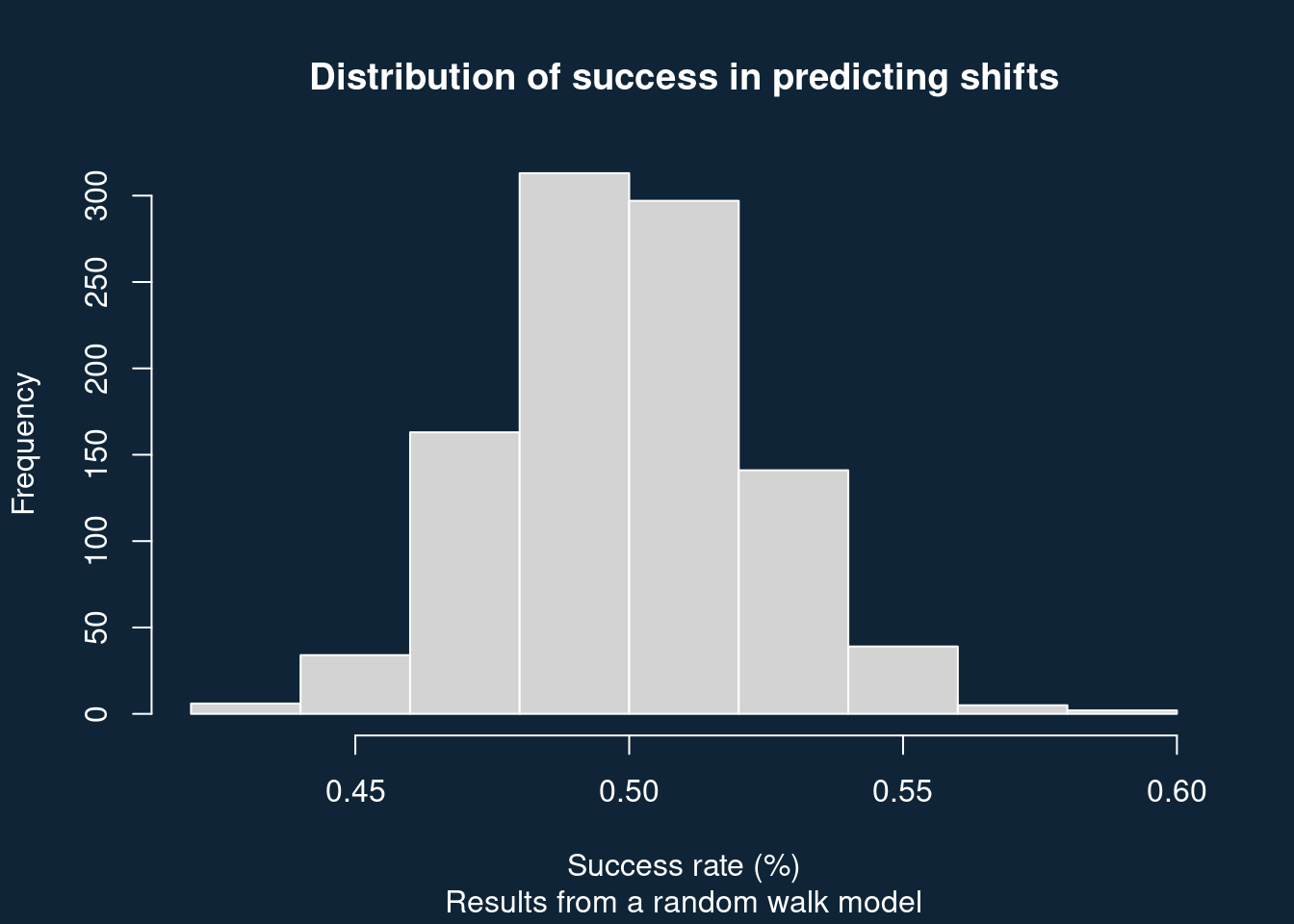
Footnotes
Because we’re using random number generation, I’ll also set a seed to make sure the results are the same across systems.↩︎